Understanding Backpropagation

Apr 2023

I’ve been working my way through Andrej Karpathy’s spelled-out intro to backpropagation, and this post is my recap of how backpropagation works. I’ll do the derivations manually first, and then write them out in code after.

1. Computational Graph

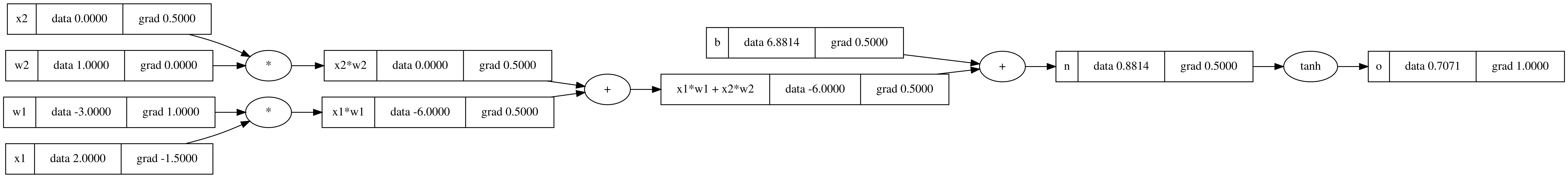
First, let’s look at a computation graph that represents the expression we’ll be looking at in this post (click on the image to see a larger version).

backprop1

This can be represented by the following expressions:

$x1w1=x1*w1$

$x2w2=x2*w2$

$x1w1x2w2=x1w1+x2w2$

$n=x1w1x2w2+b$

$o=\tanh(n)$

where

$x1=2, x2=0, w1=-3, w2=1, b=6.88$

Now that we have our expression, we’re going to do backpropagation manually.

2. Backpropagation manually

We will be calculating the gradients for each node in our computation graph with respect to o. Intuitively, this means, if we slightly change one of our inputs, how would that affect the output?

First, what is the derivative of o with respect to o? That’s simply 1.

$\frac{\partial o}{\partial o}=1$

Next, what is the derivative of n with respect to o? This is the derivative of the tanh function. There are a few different ways to do this, this is one way to do it.

$\frac{\partial o}{\partial n}=1-\tanh(o)^2=1-0.707^2=0.5$

Next, what is the derivative of x1w1x2w2 with respect to o? Because this expression is addition (+), you can think of addition operators as passing on the derivatives from the later expression. The above expression was calcualted as 0.5, so the derivative of x1w1x2w2 and b will both be 0.5.

$\frac{\partial o}{\partial x1w1x2w2}=0.5$

$\frac{\partial o}{\partial b}=0.5$

What about the derivatives for x1w1 and x2w2? Again, these are addition operations, so they are taking on the derivative from the downstream operation, 0.5.

$\frac{\partial o}{\partial x2w2}=0.5$

$\frac{\partial o}{\partial x1w1}=0.5$

Finally, we reach our inputs. The derivative of w2 with respect to o requires the chain rule. I found this intuitive explanation to be helpful in understanding what’s happening here:

As put by George F. Simmons: “if a car travels twice as fast as a bicycle and the bicycle is four times as fast as a walking man, then the car travels 2 × 4 = 8 times as fast as the man.

The essence of the chain rule is multiplying the derivatives of two or more differentiable functions. Back to our example, for w2, we need to multiply:

derivative of x2w2 with respect to o
derivative of w2 with respect to x2w2 (which is x2)

$\frac{\partial o}{\partial w2}=\frac{\partial o}{\partial x2w2}*\frac{\partial x2w2}{\partial w2}=0.5*0=0$

The same logic applies to x2. To get the derivative of x2 with respect to o, we are multiplying:

derivative of x2w2 with respect to o
derivative of x2 with respect to x2w2 (which is w2)

$\frac{\partial o}{\partial x2}=\frac{\partial o}{\partial x2w2}*\frac{\partial x2w2}{\partial x2}=0.5*1=0.5$

For the derivative of x1 with respect to o, we’re multiplying:

derivative of x1w1 with respect to o
derivative of x1 with respect to x1w1 (which is w1)

$\frac{\partial o}{\partial x1}=\frac{\partial o}{\partial x1w1}*\frac{\partial x1w1}{\partial x1}=0.5*-3=-1.5$

Finally, to get the derivative of w1 with respect to o, we need to multiply:

derivative of x1w1 with respect to o
derivative of w1 with respect to x1w1 (which is x1)

$\frac{\partial o}{\partial w1}=\frac{\partial o}{\partial x1w1}*\frac{\partial x1w1}{\partial w1}=0.5*2=1.0$

With all the derivatives in place, we can update our computation graph with the gradients for each node (click on the image to see a larger version).

backprop2

3. Backpropagation in code

Next, we’ll do the same thing but in code.

Here is our we’re going to initialize our

inputs
weights
bias
and final expression

You can see that we’re initializing values using a Value class. This class is going to hold all of our logic.

# inputs x1,x2
x1 = Value(2.0, label='x1')
x2 = Value(0.0, label='x2')

# weights w1,w2
w1 = Value(-3.0, label='w1')
w2 = Value(1.0, label='w2')

# bias of the neuron
b = Value(6.8813735870195432, label='b')

# x1*w1 + x2*w2 + b
x1w1 = x1*w1; x1w1.label = 'x1*w1'
x2w2 = x2*w2; x2w2.label = 'x2*w2'
x1w1x2w2 = x1w1 + x2w2; x1w1x2w2.label = 'x1*w1 + x2*w2'

n = x1w1x2w2 + b; n.label = 'n'

# output
o = n.tanh(); o.label = 'o'

All the code below will be part of the Value class. First off, we’re going to initialize the class. It will take in 4 params:

data: the raw value
children: the nodes that are left of the current node in the above computational graph
op: mathematical operation
label: what we see when we print it out

class Value:
  # ...
  def __init__(self, data, _children=(), _op='', label=''):
    self.data = data
    self.grad = 0.0
    self._backward = lambda: None
    self._prev = set(_children)
    self._op = _op
    self.label = label

  def __repr__(self):
    return f"Value(data={self.data})"

The above code will let us set values like: x1 = Value(2.0, label='x1'). Now that we are able to set our values for each node, we want to be able to calculate the gradient for each node. This time, instead of writing the code for each node, we will write the code for each operation.

Let’s start with the addition operation. The __add__ function states how the class should behave when it is being added with something else. In this case, we’re adding the data of the current class and other class. Once we have out, we append the _backward function onto it and return it.

The _backward function calculates the gradient for itself, and the other class that is added to it to create out. And what is the gradient/derivative calculation for an addition operation? It’s basically passing on the output’s gradient to itself and other, as we saw when we calculated it manually.

class Value:
  # ...
  def __add__(self, other):
    out = Value(self.data + other.data, (self, other), '+')

    def _backward():
      self.grad += 1.0 * out.grad
      other.grad += 1.0 * out.grad
    out._backward = _backward

    return out

The next operation is multiplication. To get the gradient, we multiply the gradient of out by other.data. And the same process with other.grad.

class Value:
  # ...
  def __mul__(self, other):
    out = Value(self.data * other.data, (self, other), '*')

    def _backward():
      self.grad += other.data * out.grad
      other.grad += self.data * out.grad
    out._backward = _backward

    return out

The last operation we’ll look at is tahnh. The calculation for the _backward is the same as what we did manually above.

class Value:
  # ...
  def tanh(self):
    x = self.data
    t = (math.exp(2*x) - 1)/(math.exp(2*x) + 1)
    out = Value(t, (self, ), 'tanh')

    def _backward():
      self.grad += (1 - t**2) * out.grad
    out._backward = _backward

    return out

The last function we’ll be writing is the backward function for the output. This is different from the above _backward functions because those ones are for specific operations. This backward function is called on the output, which calls _backward on each node.

So we need a function to traverse through all the nodes in order. The build_topo function does topological sorting:

visit each children of the current node
when all the children have been visited, add the parent node to the list

Once we have the ordered list of nodes, we will call _backward on each one, starting with the output node.

class Value:
  # ...
  def backward(self):

    topo = []
    visited = set()
    def build_topo(v):
      if v not in visited:
        visited.add(v)
        for child in v._prev:
          build_topo(child)
        topo.append(v)
    build_topo(self)

    self.grad = 1.0
    for node in reversed(topo):
      node._backward()

o.backward()

Have some thoughts on this post? Reply with an email.

Understanding Backpropagation

Contents

1. Computational Graph

2. Backpropagation manually

3. Backpropagation in code