Why understanding B-trees will help you improve database performance
Contents
1. Why are B-trees important?

Have you ever wondered why database indexes work and why they don’t work (leading to slower query times)? This post will talk about the B-tree index, the most common type of index (data structure) used to speed up query performance. With a lookup in a B-tree taking O(log n) time compared to O(n) time without an index, you’ll understand from first principles why it works. With that understanding, you’ll also figure out the situations where it won’t work.
You may even come to think that using indexes without understanding them is like driving a car without knowing how to turn. You’ll go fast, but you won’t how to prevent it from crashing.
2. What is a B-tree?

Figure 1: Designing Data Intensive Applications, Martin Kleppman, Figure 3.6
A B-tree is a tree data structure that is self-balancing. You can see that each node has more than two children, allowing for a relatively smaller tree depth that can hold a large number of nodes.
How does a lookup in a B-tree work?
- Begin at the root node
- Using the node’s trees, find the child node that would contain the search key you want
- Traverse the tree using the logic from the second step
- If you find a leaf node that has the key you want, stop. If there is no leaf node for that key or the leaf node doesn’t contain that key, return a message that the key doesn’t exist.
3. Why are B-trees used in database indexes?
Database indexes use a variety of different strategies and data structures. If you don’t specify which one to use, it will default to B-trees.
If you search for a record in a database, without an index, the search takes on average O(n) time. But if you use a database index (B-tree), then it allows for search, insertion and deletion in O(log n) (logarithmic) time (on average)!1
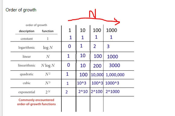
As a reminder, O(log n) means that time increases linearly while the N increases exponentially. And O(n) means that time increases exponentially while N increases exponentially.

A related and amazing aspect of B-trees is that logarithmic growth lets the tree’s number of nodes grow exponentially compared to it’s depth. In this example where each node holds 4 entries, at a tree depth of 10 you can search over 1 million records!2
| Tree Depth | Index Entries |
|---|---|
| 3 | 64 |
| 4 | 256 |
| 5 | 1,024 |
| 6 | 4,096 |
| 7 | 16,384 |
| 8 | 65,536 |
| 9 | 262,144 |
| 10 | 1,048,576 |
4. What are the implications when querying a database index?
The obvious one is that when you’re querying the database, you want to use columns that have an index. Or create an index for the column(s) that you commonly query.
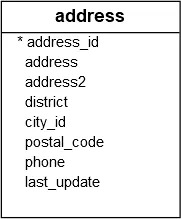
In this example, we have a table address (we’ll be using the pagila sample database for PostgreSQL).

We’ll create an index on the city_id column and query it.
create index idx_city_id on address(city_id);
select * from address where city_id = '300';
Because there is an index on the column city_id, the database will scan the index rather than the individual rows for lookup.
Bitmap Heap Scan on address (cost=4.29..9.32 rows=2 width=63) (actual time=0.020..0.021 rows=2 loops=1) Recheck Cond: (city_id = 300) Heap Blocks: exact=1 -> Bitmap Index Scan on idx_fk_city_id (cost=0.00..4.29 rows=2 width=0) (actual time=0.013..0.014 rows=2 loops=1) Index Cond: (city_id = 300)Here you can see that it is using an index scan.
a. 2-column search?
What happens if we need to search for something in 2 columns, but we only have an index in one? Continuing with the above address table example…
explain analyze select * from address where address = '47 MySakila Drive' and city_id = 300;We have an index on the city_id column, but none on the address column.
Bitmap Heap Scan on address (cost=4.29..9.32 rows=1 width=63) (actual time=0.061..0.065 rows=1 loops=1) Recheck Cond: (city_id = 300) Filter: (address = '47 MySakila Drive'::text) Rows Removed by Filter: 1 Heap Blocks: exact=1 -> Bitmap Index Scan on idx_fk_city_id (cost=0.00..4.29 rows=2 width=0) (actual time=0.040..0.041 rows=2 loops=1) Index Cond: (city_id = 300)You can see that it does do a (bitmap) index scan, while filtering for the specific address that we specify in the other column.
b. Search with a function?
What if we want to do a search using a function? In this example, we’ll use abs() on city_id.
explain analyze select * from address where abs(city_Id) = abs(300);Seq Scan on address (cost=0.00..17.05 rows=3 width=63) (actual time=0.025..0.287 rows=2 loops=1) Filter: (abs(city_id) = 300) Rows Removed by Filter: 601Planning Time: 0.221 msExecution Time: 0.323 msWe can see that it does a Seq Scan rather than use the index! Why? This is because the index only stores the values of city_id. If you use a function on city_id, then the index is not useful. But, if you do these function-based queries often, you can create a function-based index that will only be used with that specific function.
Here’s how you can create a function based index:
create index idx_abs_city_id_address on address (abs(city_id));This index will only be used when you’re using abs on city_id.
c. Partial indexes?
What if we mostly query a subset of a column and want to speed that up? For example, if we mostly look for district 'Texas', then we can create an index that will only speed up those queries.
create index idx_partial_adddress_district on address(district)where district = 'Texas';
explain analyze          select * from address          where district = 'Texas' and postal_code = '18743';
You can see that it’s using our newly created index idx_partial_address_district:
Bitmap Heap Scan on address (cost=8.16..15.75 rows=1 width=63) (actual time=0.151..0.172 rows=1 loops=1) Recheck Cond: (district = 'Texas'::text) Filter: (postal_code = '18743'::text) Rows Removed by Filter: 4 Heap Blocks: exact=5 -> Bitmap Index Scan on idx_partial_adddress_district (cost=0.00..8.16 rows=5 width=0) (actual time=0.125..0.126 rows=5 loops=1)If we use any other district, it won’t use that index:
explain analyze select * from addresswhere district = 'California' and postal_code = '18743';It instead does a sequential scan on the whole table which is much slower.
Seq Scan on address (cost=0.00..17.05 rows=1 width=63) (actual time=0.271..0.274 rows=0 loops=1) Filter: ((district = 'California'::text) AND (postal_code = '18743'::text)) Rows Removed by Filter: 6035. Summary and resources
Database indexes are not 🪄magic, they are backed by a data structure (B-trees in many cases). By understanding this, we can better reason why indexes work, and why they won’t work in certain situations (eg. function-based queries).
Resources
Footnotes
Have some thoughts on this post? Reply with an email.